Abstract

At the official request of a national Fish and Wildlife Department of one of our member countries, the European Bowhunting Federation (EBF) Scientific Committee conducted a controlled field experiment to determine the maximum range of a modern hunting arrow, both with a field point and a fixed-blade broadhead. Despite anecdotal claims, no rigorous, peer-reviewed data existed on the real-world range of arrows equipped with hunting points. Understanding maximum range is essential not only for bowhunter safety but also for guiding regulatory frameworks and land-use decisions. This study focuses on the external ballistics of hunting arrows, specifically computing aerodynamic properties that influence performance and safety.

Using a 75 lbs Mathews V3X compound bow and standardized arrows, test shots were conducted at an optimal angle (~39°) in controlled environmental conditions in Hälä, Sweden. Laser rangefinders, high-precision chronographs, and elevation instruments ensured accurate data collection. Custom Python-based simulation software was developed to calculate aerodynamic drag coefficients and verify maximum range via numerical modeling.

Results showed that arrows with field points reached an average maximum distance of 376.6 meters (Cd ≈ 1.43), while those with broadheads reached 340.1 meters (Cd ≈ 1.77). Simulations further showed that the optimal launch angles for maximum range were 39.43° (field point) and 38.72° (broadhead), validating the chosen test angle resulting in a theoretical maximal distance of respectively 396.57 m and 359.96 m. Horizontal shot scenarios demonstrated significantly shorter travel distances with a typical hunting arrow shot horizontally on the ground reaching ± 50 - 60 meter before burying itself in the ground.

This experiment provides the first quantified and scientifically validated data on real-world arrow range using broadheads. It offers a foundation for informed legislation, improved safety margins, and continued development of ballistic models for bowhunting applications.

1. Introduction

At the official request of the Fish and Wildlife department of one of our member nations what the maximal range of an arrow equipped with a hunting point is, the European Bowhunting Federation (EBF) Scientific committee set out to answer this question with a detailed field experiment. Although anecdotical data on this kind of data exist, no well documented and reliable data were available. This question is not just a matter of curiosity, it’s important for both hunter safety and regulatory frameworks.

When discussing the legalization and regulation of bowhunting, authorities must understand effective range and safety margins involved. The maximum range of a hunting arrow, especially when equipped with a hunting point, is a key factor in determining safe hunting practices and legal requirements. Although it all drills down to common sense, still it is useful to perform a controlled test especially because there was no reliable data in the scientific literature regarding the real-world range of arrows with broadheads. This gap prompted the EBF Scientific committee to design and execute a controlled experiment to provide concrete answers.

The experiment had two main objectives:

1. Determine the maximum range of a hunting arrow, both with a practice field point and with a broadhead.
2. Measure the aerodynamic drag coefficient (Cd) of a standard hunting arrow to ensure accurate simulations.

These insights are essential for both practical bowhunting knowledge and for informing policymakers and legislators.

2. Bow and arrows used

2.1 Bow and Arrow Specifications

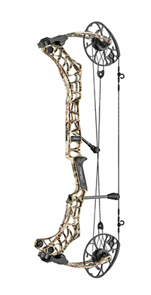
• Mathews V3X, 75 lbs compound bow
• Arrow weight (Field Point): 495.22 grain / 32.09 g avg.
• Arrow weight (Broadhead): 496.46 grain / 32.17 g avg.
• Launch velocity: ~291 fps / 88.70 m/s (both arrow types)
• Arrow kinetic energy at launch: 126.54 J

3. Test Conditions

3.1 Location:

• Hölö, Sweden, with a safe 700 m shooting lane
• 40 meter above sea level for shooting and landing position

3.2 Weather:

• 4°C temperature
• Wind 19 km/h SSW
• 81% humidity
• Air pressure 982 mb
• Air density 1.231 kg/m³

4. How to estimate arrow drag?

The aerodynamic drag coefficient (𝐶𝑑) is determined by the arrow’s shape and surface characteristics and quantifies the amount of air resistance it encounters during its trajectory. It serves as the foundation for calculating the ballistic coefficient of any projectile, including rifle bullets. The drag force experienced by a projectile (like an arrow or bullet) moving through air is given by the equation:

Where:

• ρ is air density in kg/m³
• v is arrow speed in m/s
• A is cross-sectional area in m² 
• Cd is the drag coefficient

The higher the Cd value, the more resistance the arrow will experience when shot through air (or any medium); similar; lower Cd values result in lower resistance force (drag) experienced.

With no published values for arrows equipped with hunting broadheads, an experiment was needed to estimate Cd  based on actual trajectory data.

5. Software development

To precisely calculate the trajectory of an arrow under realistic conditions, custom simulation software simulating the trajectory of a point-mass was developed in Python language. The core of this program numerically solves the equations of motion for an arrow in three dimensions. The model accounts for gravity and aerodynamic drag, while allowing the user to specify real-world parameters such as arrow mass, drag coefficient, launch angle, wind speed and direction. It can also include optional Coriolis effects caused by the Earth’s rotation. The drag force is calculated based on the standard equation shown above where all terms, including air density and cross-sectional area, are explicitly set in the software.

Since the drag force makes the equations impossible to solve analytically, the script uses a numerical approach: it employs the solve_ivp function from the SciPy [1] library with the RK45 method, a 5th order (global accuracy) adaptive Runge-Kutta integrator that uses an embedded 4th-order method for adaptive step size control [2]. The simulation continues stepwise until the arrow returns to the ground or reaches a user-specified target height. All key outcomes, such as range, time of flight, impact velocity and kinetic energy, are computed and printed, and the entire 3D trajectory can be visualized thanks to built-in plotting routines. This robust computational approach allows researchers to realistically model the performance of hunting arrows under a wide range of physical and environmental conditions, supporting both experimental analysis and practical recommendations for the field.

The authors acknowledge that the use of a point-mass simulation represents a simplification of real-world arrow flight dynamics. More advanced approaches, such as six-degree-of-freedom (6-DoF) modeling that accounts for arrow spin stabilization, center of pressure shifts, yaw of repose, and effects like the Magnus force, would offer higher-fidelity simulations. However, given the relatively short range of hunting arrows and the predominantly stable, near-axisymmetric flight conditions observed in practice, this simplified model is considered sufficient for the objectives of this study and is not expected to introduce significant bias in the results.

It is important to note that the current simulation assumes a constant drag coefficient throughout the arrow’s flight. In reality, the drag coefficient is velocity-dependent, particularly in the subsonic regime typical of arrow speeds. As the arrow decelerates due to aerodynamic drag, the Reynolds number decreases, which can lead to moderate variations in 𝐶d, especially for arrows with complex geometries such as broadheads and fletching. While this simplification is considered acceptable for the scope of this study, focused on general range and safety estimations, it may introduce small deviations in the computed trajectories, particularly over longer flight distances. Incorporating a velocity-dependent drag coefficient could refine the model and will be considered in future analyses for improved precision.

6. The Experiment: Measuring Maximum Range

To ensure reproducible and realistic results, the team sought to launch arrows as close as possible to the optimal angle for maximum distance, calculated initially using estimated Cd values from previous short-range tests where velocities were measured at launch and at 24.5 meter. From these experiments the drag coefficient was estimated to be around 1.62. (Data not shown and available upon request.)

Based on this initial estimated drag coefficient, the optimal launch angle was calculated and arrows were shot at ~39°, the theoretically optimal angle, and their landing points were precisely measured.

With the lack of a shooting robot, in order to be as close to the set 39° angle, a frame was constructed with a known 39° inclination that allowed the arrow to be aligned to this reference. This proved to be very efficient (see further at the results section).

Using publicly available LIDAR elevation data for the area, confirmed on site with a rotating laser, the difference in height between the launch point and the arrow landing zone was found to be 20 cm. This minimal elevation change makes the site ideally suited for these kinds of ballistic tests.

7. Key Measurements and Results

7.1 Range Results

For each of the conditions, 2x 5 arrows were shot, so 10 datapoints per condition. This resulted in the following distances:

• Field Points:
  • Average Maximum Range: 376.6 meters
  • Consistency: ±3.6 m (0.96%) –
• Broadheads:
  • Average Maximum Range: 340.1 meters
  • Consistency: ±5.3 m (1.56%)

8. Calculating the Drag Coefficient

By matching the measured ranges to the expected arrow trajectories, the team deduced the effective drag coefficients by entering the physical properties of the arrow and obtained distances in the simulation software and optimizing for the drag coefficient.  This was done using the brentq method of the root_scalar function of the Scipy [1] package. This resulted in the following values:

• Field Point Arrow: Cd = 1.43 ± 1.3% instrument error
• Broadhead Arrow: Cd = 1.77 ± 1.3% instrument error

As expected, broadheads increase drag, reducing arrow range. Field points were used as a 'best-case scenario' substitute for mechanical broadheads. The majority of hunting arrows will have Cd values within this range. While using three low-profile vanes can reduce drag, it may compromise aerodynamic stability, particularly when shooting mechanical or fixed broadheads that induce their own aerodynamic steering.

The drag coefficients were calculated assuming a 19 km/h south-southwest (SSW) wind. Since the aim of this study was to determine the maximum range of a typical hunting arrow, the wind was factored into the drag coefficient estimation. This approach may lead to a slight underestimation of the actual drag coefficient, and consequently, a slight overestimation of the arrow’s maximal range. However, this overestimation errs on the side of safety, providing a conservative upper bound that is more suitable for evaluating potential long-range scenarios in the field.

9. Simulations

By modeling the external ballistics of arrows at various launch angles and using experimentally determined drag coefficients, we conducted simulations to address both practical and safety-relevant questions, such as identifying the optimal launch angle for maximum range, and estimating how far a hunting arrow travels when fired horizontally.

9.1 Optimal Launch Angles

With these newly calculated drag coefficients, we can compute the optimal launch angle for maximum trajectory range. Again, by entering the physical properties of the arrow into the software and optimizing which launch lange would yield the longest shot, the following values were obtained.

• Field Point: 39.429°
  • 396.57 m max range ± 2.3 m 
  • 37.80 J kinetic energy at impact (29.94% of the initial kinetic energy)
• Broadhead: 38.724°
  • 359.96 m max range ± 2.3 m
  • 32.76 J kinetic energy at impact (25.82% of the initial kinetic energy)

For these calculations and finding the optimal angle, the brent method of the minimize_scalar function of the Scipy[1] package was used.

These results show that our initial calculation of 39° was very good and in between both optimal values! 

The hunting arrow used in this study was purpose-built to ensure aerodynamic stability and consistent aerodynamic behavior. The 4x fletching design intentionally increases lift, which contributes to stabilizing the arrow’s trajectory, albeit at the cost of increased aerodynamic drag. Despite this trade-off, simulations show that even under favorable conditions with a low drag coefficient (as low as e.g. 1), the arrow's maximum range remains below 475 meters. This underscores the inherent limitations on the maximum range of hunting arrows, imposed by their high drag-to-mass ratio, even in optimized configurations.

9.2 Horizontal shots:

Although broadhead-equipped arrows should always be shot in a downward trajectory, ensuring they embed safely into the ground, a hillside, or the terrain below, as is typically the case when shooting from a treestand, elevated platform, or even when standing on level ground, it remains crucial to understand how far a hunting arrow can travel if accidentally released on a horizontal path.

By using the obtained drag coefficients, arrow trajectories were calculated for a zero degree launch angle, starting at 1.6 meter high (average person standing up) or from 7.6 meters high (shooting from a treestand position at 6 meters high). These are the results obtained for both fieldpoint or broadhead equipped hunting arrows.

• Horizontal launches - From ground (the arrow starts at a height of 1.6 meter):
  • Field Point: 49.0 m
  • Broadhead: 48.7 m
• From a treestand positioned at 6 meter (the arrow starts at a height of 7.6 meter):
  • Field Point: 103.0 m
  • Broadhead: 101.5 m

9.3 Trajectories for real world hunting situations

In typical hunting situations, the bow hunter will be positioned in a treestand or or from high position and hunt at distances around 20 meters. So the plot clearly indicates that these are always shot angles by which the arrow will bury itself in the ground very close to the target. The indicated distance is the horizontal distance from the base of the tree or platform to the target.

10. Conclusions: What Did We Learn?

• A modern hunting arrow from a 75# compound bow can, at best, travel up to ± 400 meters (field point) or ± 360 meters (broadhead) when shot at the optimal angle. Most bowhunters will hunt with a 70# bow or lower. So the 75# is above average upper boundary and was chosen for this reason.
• The presence of a fixed broadhead increases drag and reduces maximum range.
• Even under ideal (and unrealistic) conditions, the range is much less than a rifle bullet, but well beyond typical bowhunting distances.
• Having developed ballistic software capable to accurately predict hunting arrow trajectories enables us to answer many more questions and simulate e.g. light versus heavy arrow trajectories and calculate the kinetic energy at impact. This might be the subject of another article.

11. Implications for Bowhunters and Legislation

These results provide science-based evidence for policy-makers, helping to establish safe buffer zones, define legal hunting parameters, and promote responsible bowhunting practices. 

For hunters, the data underscores the importance of understanding arrow ballistics, especially regarding safe shooting angles and ensuring that the arrow will bury itself after the shot.

12. Conclusion on Maximum Range and Safety Considerations

The results of this study indicate that the tested hunting arrow, under optimal launch conditions, has a maximum range of approximately 360 meters. It also confirms that arrows shot from elevated positions pose virtually no risk beyond the intended target, due to their steep downward trajectory.

In contrast, a big game rifle bullet can travel more than ten times that distance, and modern monometal bullets in particular carry a significant risk of ricochet. This stark difference highlights the inherently safer nature of bowhunting in terms of stray projectile hazards.

13. Validation of Arrow Flight Model via Analytical Terminal Velocity Comparison 

To validate the accuracy of the arrow flight simulation model, we compared the terminal velocity obtained from the numerical simulation to the analytically derived terminal velocity using the standard drag equation. The theoretical terminal velocity is given by:

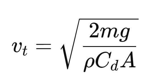
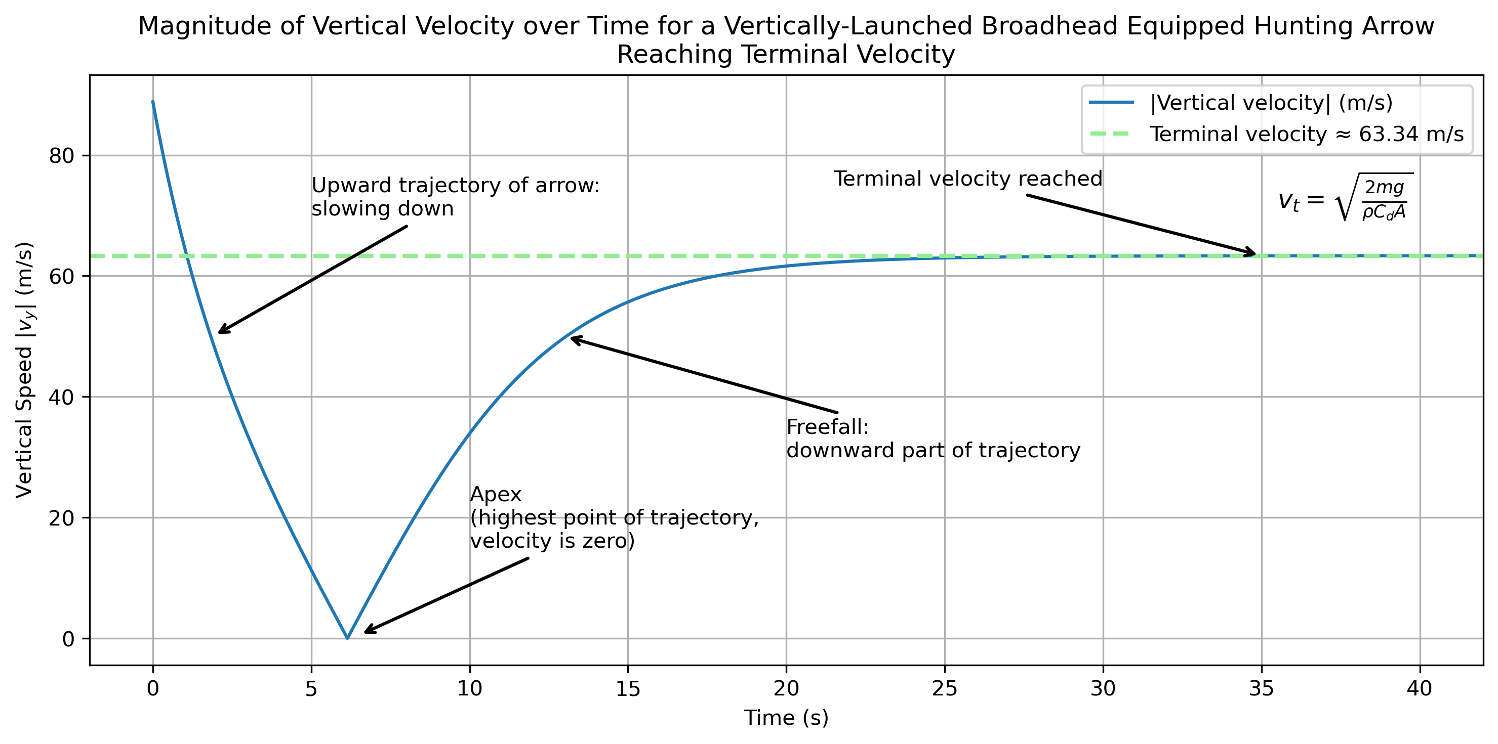
where m is the arrow mass, g is the gravitational acceleration, ρ is the air density, Cd is the drag coefficient, and A is the arrow's frontal surface area (including vanes). The simulation was configured with a vertical launch angle and a sufficiently high release altitude (2000 m) to ensure enough flight time for the arrow to reach terminal velocity. The simulated vertical velocity curve shows a plateau phase in the descending part of the trajectory, corresponding to a terminal velocity of approximately 63.34 m/s. This value is in near-perfect agreement with the analytically computed terminal velocity of 63.34 m/s, confirming that the simulation faithfully reproduces the physics of free-falling drag-limited motion. This match between numerical and theoretical results serves as a strong internal validation of the model, especially in the aerodynamic regime where drag dominates motion.

The figure below shows the magnitude of the vertical velocity of a vertically launched broadhead-equipped hunting arrow as a function of time. The arrow is launched straight upward at approximately 291.4 fps (88.8 m/s) from a height of 2000 m. The trajectory exhibits a typical ballistic profile: during the initial ascent, the vertical speed decreases due to gravitational deceleration and aerodynamic drag. The apex, where vertical velocity momentarily reaches zero, occurs around 6.14 seconds after launch. This is followed by the descent phase, during which the arrow accelerates downward under gravity until the opposing drag force balances out the gravitational pull. Beyond this point, the arrow reaches its terminal velocity, clearly visible in the plot as a plateau, which stabilizes around 63.34 m/s (207.81 fps). This value closely matches the analytically predicted terminal velocity, further validating the accuracy of the implemented flight model. Annotations are added to highlight key phases of the trajectory: the deceleration during ascent, the apex, the free-fall acceleration, and the onset of terminal velocity. The horizontal dashed line represents the theoretical terminal velocity derived from physical parameters such as drag coefficient, air density, cross-sectional area, and mass.

14. Acknowledgements

This experiment was made possible through the efforts of the EBF scientific committee, with special thanks to Olof Reinhammar and Anders Geier for preparing the equipment and doing the shooting tests; Luc Krols for writing the python scientific software code and doing the calculations.

Field data collected January 15th, 2023. For the full scientific report and raw data, contact the European Bowhunting Federation.

15. Appendix: Equipment and tools used

15.1 Detailed Bow and Arrow Specifications

• Bow:
  • Mathews V3X, 29" compound bow
  • 75 lbs draw weight, an above average draw weight
  • 29.5” draw length,
  • International Bowhunting Organization / IBO rating: 340 fps
  • 126.54 Joules kinetic energy
• Arrow:
  • Carbon shaft: 5 mm inner diameter, 6.82 mm outer diameter, 250 spine
    • Total length including field point: 796 mm / 31.34”
    • Total length including field point: 816 mm / 32.14”
  • Fletching:
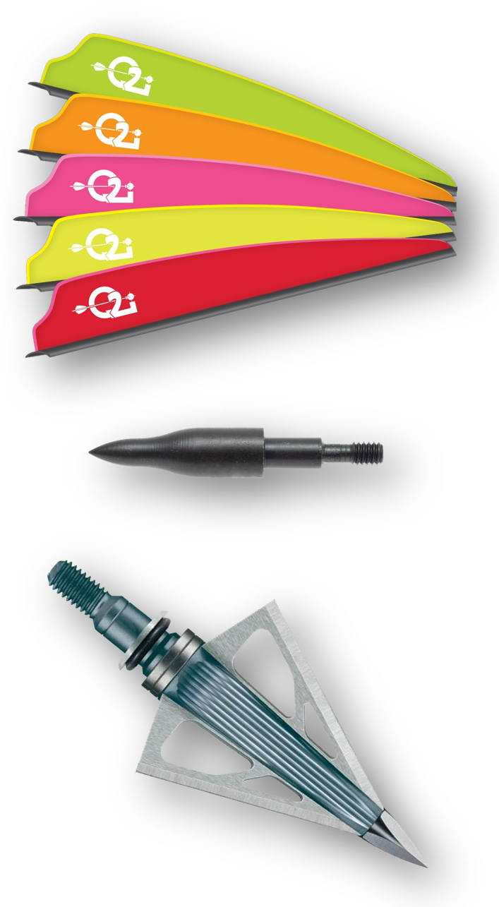
    • Four 2.1” Q2i Archery Fusion Zeon X-II vanes
      • Length: 2.1” / 53.34 mm
      • Height: 0.44” / 11.176 mm
      • Width: 0.0315” / 0.8001 mm
      • Weight: 5.5 grains / 0.3564 gram
    • Helical fletched at ~3°
  • Points:
    • Saunders Combo 21/64” 125 grain / 8.10 gram field point
    • New Archery Products Thunderhead 125 grain / 8.10 gram broadhead

15.2 Measurement tools

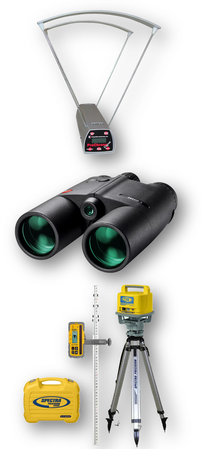• Chronograph:
  • Competition Electronics ProChrono Digital
  • 0.5% accuracy
• Distance meter:
  • Leica Geovid 2200 laser binoculars
  • Accurary: ±1 m up to 500 meters
• Elevation measurement
  • Spectra Precision Laser HL700 rotary laser receiver
  • Accuracy ±1m < 500 meter
• Scale
  • Last Chance Archery Pro Grain Scale 2.0
  • Accuracy 0.01g / 0.15 grain

15.3 Arrow Weights and Velocity

• Arrow weight (Field Point): 495.22 grain / 32.09 g avg.
• Arrow weight (Broadhead): 496.46 grain / 32.17 g avg.
• Launch velocity: ~291 fps / 88.70 m/s (both arrow types)
• Arrow kinetic energy at launch: 126.54 J

16 References:

[1]. Pauli Virtanen, Ralf Gommers, Travis E. Oliphant, Matt Haberland, Tyler Reddy, David Cournapeau, Evgeni Burovski, Pearu Peterson, Warren Weckesser, Jonathan Bright, Stéfan J. van der Walt, Matthew Brett, Joshua Wilson, K. Jarrod Millman, Nikolay Mayorov, Andrew R. J. Nelson, Eric Jones, Robert Kern, Eric Larson, CJ Carey, İlhan Polat, Yu Feng, Eric W. Moore, Jake VanderPlas, Denis Laxalde, Josef Perktold, Robert Cimrman, Ian Henriksen, E.A. Quintero, Charles R Harris, Anne M. Archibald, Antônio H. Ribeiro, Fabian Pedregosa, Paul van Mulbregt, and SciPy 1.0 Contributors. (2020) SciPy 1.0: Fundamental Algorithms for Scientific Computing in Python. Nature Methods, 17(3), 261-272. DOI: 10.1038/s41592-019-0686-2.

[2]. J. R. Dormand, P. J. Prince, “A family of embedded Runge-Kutta formulae”, Journal of Computational and Applied Mathematics, Vol. 6, No. 1, pp. 19-26, 1980. DOI: 10.1016/0771-050X(80)90013-3